Introduction

Telecom services, such as voice, data and video services are delivered on various telecommunication networks to subscriber's homes and businesses. Failures and operating problems associated with the network and network equipment cause service problems in which some of them can be fixed remotely and others require dispatch of technicians to the site to repair and fix the problem(s). Managing the available resources and their capacity in executing the repair jobs is quite challenging because the daily volume of dispatch needs (jobs demand) is largely unpredictable due to several factors such as the characteristics of the network and network equipment, nature of repairs needed, regulations, weather, seasonality, and characteristics of the labor force (such as union membership, skills, culture); among others. On the other hand, if extra resources and capacity is secured, the cost to secure these resources in addition to unplanned overtime cost can be substantial. If a lack of resources and capacity exists, then broken promises and negative customer experiences occur which typically affects customer satisfaction. The ability to predict the jobs demand in advance for immediate and near short terms can provide substantial benefits in optimizing capacity, reducing network downtime and improving customer satisfaction.

Objectives

We sought to develop a statistical model to predict the daily and 21-day period demands for telecom repair services to help in optimizing repairs resources capacity, improve operational effectiveness, reduce overtime cost and improve customer services.

Our inital hypothesis is that the number of repair jobs is related to weather conditions plus seasonality or some other time related phenomena. This project will help us identify and develop a model for repair jobs based based on this idea.

Dataset Descriptions

The Boston data included 2 years of daily measurements for actual repairs, weather data forecasts and measurements, and other repair center metadata.

Specifically We obtained raw data to be used for the model development and testing that included:

• Historical time series actual repairs dispatch job for a service area (zip code),
• Historical weather data for the geographical area covered by the repairs service center,
• Forecasted weather data for the geographical area covered by the repairs service center, and
• Metadata on the repairs center, the day of the week, and holidays

The weather data is commercially available from Accuweather and the jobs data are available from a major telecom provider for two independent geographical service areas.

• 02116 - Boston, Massachusetts
• 02865 - Lincoln, Rhode Island

Exploratory Analysis

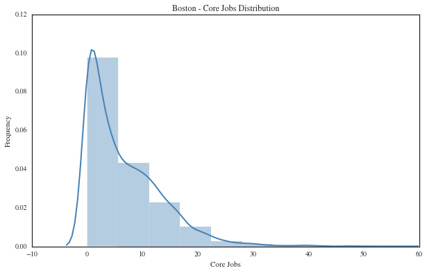
The repairs jobs data from the centers were accumulated at the group level since capacity planning is also mainly conducted at the group level. The repairs jobs data for Boston included the repairs jobs for period from 1/1/2013 to the 10/18/2014. The weather data for the same time period were previously obtained from a commercial source (Accuweather.com) and linked to the repairs jobs based on the zipcode and date.

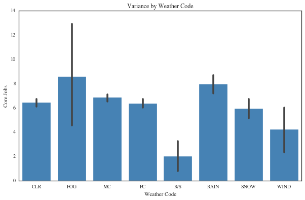
In addition to the weather measurements, a weather code is assigned to the conditions. These data are categorical and can be transformed to dummy variables so that their relationship to corejobs can be explored. The weather codes and their description are below.

• CLR : clear conditions
• FOG : foggy
• MC : mostly cloudy
• PC : partly cloudy
• R/S : rain/snow
• RAIN : raining
• SNOW : snowing
• WIND : elevated wind gusts

Also included in the dataset is a categorization about type of holiday. The above chart shows separatation of corejobs number by type of major holiday. Holiday type appears to help separate repair jobs demand. Holiday types can be broken down into:

• H = holiday (most federal holidays including patriot's day, columbus day, etc.)
• M = major holiday (new year, july 4th, thanksgiving, christmas, etc.)
• N = non-holiday

Feature Selection

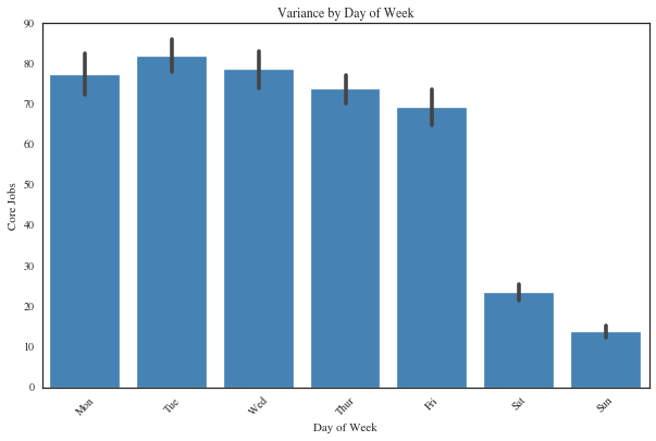
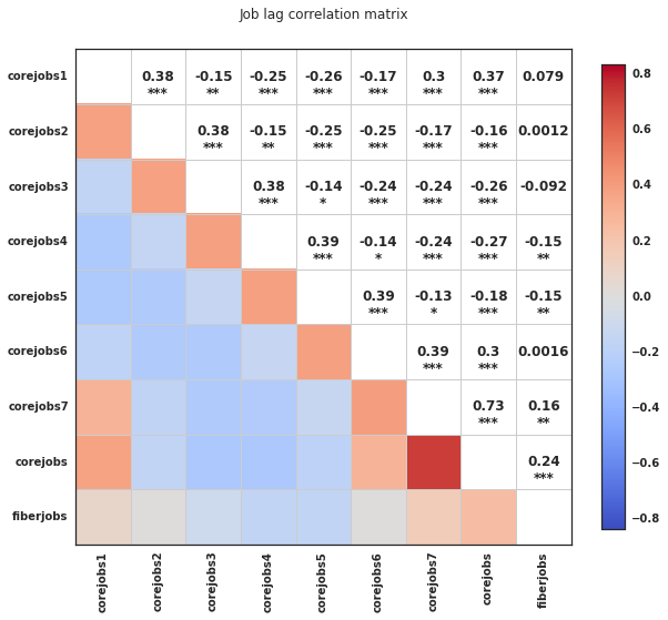
Our findings included observing a repeated pattern in the number of repairs jobs within the week preceding any specific day. This pattern, where the jobs counts are higher during the first three days of the week (peak), taper down toward the weekend, and become lower within the weekend (valley) led to the creation of more features that we are calling 'jobs-days-lags' as input variables for modeling. Further, there were correlations not only for the weekdays versus weekends but also within the weekdays themselves so dummy variables for each day of the week were selected as input for the model development.

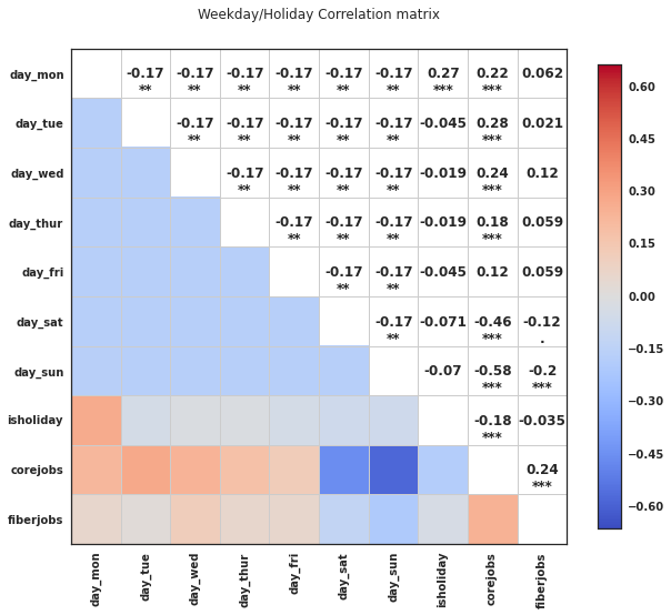
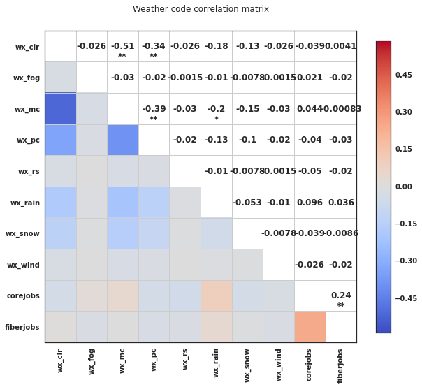
Analysis of the holiday’s impact on the jobs also indicated a pattern of reduction during the day of the holiday and because we've seen a normal pattern of previous days jobs affecting the next days jobs, we're including an indicator for the day after the holiday. Binary variables for the holiday and the day after the holiday were created and selected for input as well. Finally, extensive correlation analysis of the weather variables showed that one of the categorical variables that include weather conditions is strongly correlated with the repairs jobs. This variable was also coded into dummy variables where the set is selected as input for consideration in the model development.

We revisited our correlation analysis after exploring these categorical data and found parameters that would prove useful for linear regression modelling as can be seen in the next three charts.

Model Description

Two modeling approaches were attempted: Bayesian statistics and linear regression. The bayesian statistics did not yield any conclusive results, possibly because the data is not from a normal distribution so our efforts were focused on linear regression. Linear regression was selected because it is a better fit for the prediction problem at hand, provides opportunity to explain input drivers of the prediction to business (which is a business requirement) compared to a black box approach like neural networks, and provides manageable production implication for the model (see the note the model production deployment). Finally, the ability to use the modeling algorithm itself as a vehicle to better select the input variables was a critical consideration since the reducing the number of input variables for the model, as much as practically possible, is an important business requirement for deployment and productionalization.

The initial set of the input variables selected during the data exploration and features selection stages were employed in the linear regressions. Model optimization was performed throughout multiple steps of backward elimination where input variables are evaluated in the regression(s) and the ones that carry the least statistical significance were removed. The first step included the whole set of the initial input variables selected during the data exploration and features selection then a subsequent regression model step is exercised to remove the weakest variable from the initial set. A second step includes the whole initial set of variables minus the removed variable in the first step and likewise regression is used to remove the weakest input variables from the remaining set and so on. A total of ten steps were used to reach the final set of input variables for the final regression model. All variables elimination from the regressions was based on testing the hypothesis of no difference for the corresponding regression coefficients at the alpha level of 0.05.

The following charts show feature coefficients before and after elimination.

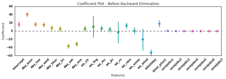
The parameters of the model that remain are day of the week, rain, holiday, day after holiday, and corejobs counts from the previous days. However it is not clear why only some of the corejobs from previous days have an effect but it could have something to do with how jobs stack up during the week and then taper off on the weekends.

Testing and Conclusions

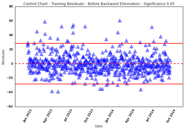
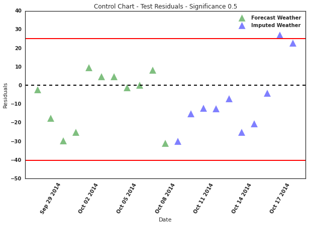
The finalized regression model is tested using the data from 9/28/2014 to 10/18/2014 to assess the model performance, establish the control chart, and structure the scoring process. The latter was divided into two parts: (1) scoring for the first 11 days, and (2) scoring for day 12 to day 21. The reason for the separate scoring is the availability of forecasted weather data for the model input. While the model prediction period is 21 days, only the first 11 days have forecasted weather data. As a result, an imputation was developed to supplement the forecasted weather data for the second period prediction. The imputation is specific to the rain variable because the final input variables included only rain from the set of weather data used during the model development process. Since rain is a binary variable (1,0), the expected value of the rain variable during the first 11-day period is used to impute the missing forecasted rain variable needed for the model in the days within the second 10-day period.

The model prediction was tested using the mean absolute pediction error (MAPE), which is the ratio of the mean absolute residuals during the 21-day predicted repairs jobs over the mean actual jobs during the same 21-day period. The business requirement for the model prediction accuracy requires a performance criterion of MAPE of less than or equal to 0.4. The linear regression developed in this project meets and exceeds the required MAPE level.

The following charts show the residual errors for both the training and testing data set.

The model developed in this project is applicable only to a specific geographical area but our process can be replicated nationwide. Our model for the Boston area data scored well enough to reliably predict job demand during our test period with an accuracy score of 73%. Below is the predicted results for our test period. It can be seen in the chart below that the model correctly predicts dips in the weekends and even preducts a reduced job demand for the Monday holiday, which is Columbus Day.